LP – Show & Sell

Problem

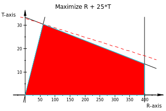
Show & Sell can advertise its products on local radio and television (TV). The advertising budget is limited to $10,000 a month. Each minute of radio advertising costs $15 and each minute ofTY commercials $300. Show & Sell likes to advertise on radio at least twice as much as on TV. In the meantime, it is not practical to use more than 400 minutes of radio advertising a month. From past experience, advertising on TV is estimated to be 25 times as effective as on radio. Determine the optimum allocation of the budget to radio and TV advertising.

OR Model

Decision variables
R: number of advertising minutes on radio per month
T: number of advertising minutes on TV per month

Objective function
Z: effectiveness of advertising that we need to maximize
Z = 25*T + R

Constraints
15*R + 300*T <= 10000
R >= 2*T
R >= 400
T <= 0

LP Graphical Solution

Using MuPad (Symbolic Math) in MATLAB:

k := [
         {15*R + 300*T <= 10000,
          R >= 2*T,
          R <= 400,
          T >= 0},
      25*T + R,
      NonNegative
    ]:
g := linopt::plot_data(k, [R, T]): plot(g):

Output:

The optimum solution is at R=60, T=30.

LP – Recycling Center

Problem

An industrial recycling center uses two scrap aluminum metals, A and B, to produce a special alloy. Scrap A contains 6% aluminum, 3% silicon, and 4 % carbon. Scrap B has 3% aluminum, 6% silicon, and 3% carbon. The costs per ton for scraps A and Bare $100 and $80, respectively. The specifications of the special alloy require that

• the aluminum content must be at least 3% and at most 6%
• the silicon content must lie between 3% and 5%
• the carbon content must be between 3% and 7%.

Determine the optimum mix of the scraps that should be used in producing 1000 tons of the alloy.

OR Model

Decision variables
A: amount of metal A
B: amount of metal B
Objective function
Z: cost of alloy

Constraints

	A	B	>	<
Al	0.06	0.03	0.03	0.06
Si	0.03	0.06	0.03	0.05
C	0.04	0.03	0.03	0.07
~	0.87	0.88	–	–

LP Graphical Solution

Using MuPad (Symbolic Math) in MATLAB:

k := [
         {(0.06*A+0.03*B) >= 0.03 * (A+B),
          (0.06*A+0.03*B) <= 0.06 * (A+B),
          (0.03*A+0.06*B) >= 0.03 * (A+B),
          (0.03*A+0.06*B) <= 0.05 * (A+B),
          (0.04*A+0.03*B) >= 0.03 * (A+B),
          (0.04*A+0.03*B) <= 0.07 * (A+B),
          A+B>=1000},
      -100*A-80*B,
      NonNegative
    ]:
g := linopt::plot_data(k, [A, B]): plot(g):

Output:

Optimal solution: A = 333.33, B = 666.66.

LP – Day Trader

Problem

Day Trader wants to invest a sum of money that would generate an annual yield of at least $10,000. Two stock groups are available: blue chips and high tech, with average annual yields of 10% and 25%, respectively. TIlOugh high-tech stocks provide higher yield, they are more risky, and Trader wants to limit the amount invested in these stocks to no more than 60% of the total investment.
What is the minimum amount Trader should invest in each stock group to accomplish the investment goal?

OR Model

Decision variables
B: investment in blue chips
T: investment in high tech

Objective function
Z: investment that we need to minimize
Z = B + T

Constraints
0.1*B + 0.25*T >= 10000,
T <= 0.6*(T+B)

LP Graphical Solution

Using MuPad (Symbolic Math) in MATLAB:

k := [
         {0.1*B + 0.25*T >= 10000,
          T <= 0.6*(T+B)},
      -T-B,
      NonNegative
    ]:
g := linopt::plot_data(k, [T, B]): plot(g):

Output:

The optimum solution is at T=31600, B=21000.

LP – Ma-and-Pa grocery store

Problem

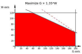
In the Ma-and-Pa grocery store, shelf space is limited and must be used effectively to increase profit. Two cereal items, Grano and Wheatie, compete for a total shelf space of 60 ft2. A box of Grano occupies 0.2 ft2 and a box of Wheatie needs 0.4 ft2. The maximum daily demands of Grano and Wheatie are 200 and 120 boxes, respectively. A box of qrano nets $1.00 in profit and a box of Wheatie $1.35.
Ma-and-Pa thinks that because the unit profit of Wheatie is 35% higher than that of Grano, Wheatie should be allocated 35% more space than Grano, which amounts to allocating about 57% to Wheatie and 43% to Grano. What do you think?

OR Model

An OR model has 3 components:

• Decision variables
  G: number of Grano boxes
  W: number of Wheatie boxes
• Objective function
  Z: objective function that we need to maximize
  Z = G + 1.35 *W
• Constraints
  0.2*G + 0.4*W <= 60
  G <= 200, G >= 0
  W <= 120, W >= 0

LP Graphical Solution

Using MuPad (Symbolic Math) in MATLAB:

k := [
         {.2*G + .4*W <= 60,
          G <= 200,
          W <= 120,
          G >= 0,
          W >= 0},
      G + 1.35*W,
      NonNegative
    ]:
g := linopt::plot_data(k, [G, W]): plot(g):

Output:

The optimum solution is at G=200, W=50.

Comment

The proposed solution ignores the space constraints. Although, Wheatie is more profitable by 35%, Grano takes half the shelf space. And as we see from the optimum solution, we’ll utilize the available allocation for Grano up to the maximum and the rest is allocated for Wheatie.

10088 – Trees on My Island

Given a polygon whose vertices are of integer coordinates (lattice points), count the number of lattice points within that polygon.
Pick’s theoreom states that
Where

• is the number of lattice points in the interior (this is our program’s output).
• is the area of the polygon.
• is the number of lattice points on the exterior.

All the reqired quantities are easily computable, however, needs some extra work. To find the number of lattice points on line segment , we simply calculate .
C++ implementation with rank 329:

#include <iostream>
#include <algorithm>
#include <complex>
#include <vector>
using namespace std;

typedef long long gtype;
typedef complex<gtype> point;
#define x real()
#define y imag()
#define crs(a, b) ( (conj(a) * (b)).y )

long double polArea(vector<point> & p) {
	long double area = 0;
	for (size_t i = 0; i < p.size() - 1; ++i)
		area += crs(p[i], p[i + 1]);
	return abs(area) * 0.5;
}

long long gcd(long long a, long long b) {
	long long t;
	while (b)
		t = b, b = a % b, a = t;
	return a;
}

long long polLatticeB(vector<point> & p) {
	long long b = 0;
	for (size_t i = 1; i < p.size(); ++i)
		b += gcd(abs(p[i].y - p[i - 1].y), abs(p[i].x - p[i - 1].x));
	return b;
}

int main() {
	int n;
	while (cin >> n && n) {
		// polygons
		vector<point> p(n + 1);
		for (int i = 0; i < n; ++i)
			cin >> p[i].x >> p[i].y;
		p[n] = p[0];
		// is convex
		cout << (long long) (polArea(p) - polLatticeB(p) * 0.5l + 1) << endl;
	}
	return 0;
}